SciPy. Matplotlib

По материалам сайта http://cs231n.github.io/python-numpy-tutorial/

SciPy

Numpy предоставляет высокопроизводительный многомерный массив и базовые инструменты для вычисления и управления этими массивами. SciPy основывается на этом и предоставляет большое количество функций, которые работают с массивными массивами и полезны для различных типов научных и инженерных приложений.

Лучший способ познакомиться с SciPy - это просмотреть документацию . Мы выделим некоторые части SciPy, которые могут оказаться полезными для этого класса.

Операции с изображениями

SciPy предоставляет несколько основных функций для работы с изображениями. Например, у него есть функции для чтения изображений с диска в массивы, для записи на диск массива в виде изображений и для изменения размера изображений. Вот простой пример, который демонстрирует эти функции:

from scipy.misc import imread, imsave, imresize

# Read an JPEG image into a numpy array
img = imread('assets/cat.jpg')
print(img.dtype, img.shape)  # Prints "uint8 (400, 248, 3)"

# We can tint the image by scaling each of the color channels
# by a different scalar constant. The image has shape (400, 248, 3);
# we multiply it by the array [1, 0.95, 0.9] of shape (3,);
# numpy broadcasting means that this leaves the red channel unchanged,
# and multiplies the green and blue channels by 0.95 and 0.9
# respectively.
img_tinted = img * [1, 0.95, 0.9]

# Resize the tinted image to be 300 by 300 pixels.
img_tinted = imresize(img_tinted, (300, 300))

# Write the tinted image back to disk
imsave('assets/cat_tinted.jpg', img_tinted)

 

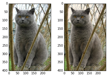
Слева: исходное изображение. Справа: тонированное и измененное изображение.

Файлы MATLAB

Функции scipy.io.loadmatи scipy.io.savematпозволяют читать и писать файлы MATLAB. Вы можете прочитать о них в документации .

Расстояние между точками

SciPy определяет некоторые полезные функции для вычисления расстояний между наборами точек.

Функция scipy.spatial.distance.pdistвычисляет расстояние между всеми парами точек в данном наборе:

import numpy as np
from scipy.spatial.distance import pdist, squareform

# Create the following array where each row is a point in 2D space:
# [[0 1]
#  [1 0]
#  [2 0]]
x = np.array([[0, 1], [1, 0], [2, 0]])
print(x)

# Compute the Euclidean distance between all rows of x.
# d[i, j] is the Euclidean distance between x[i, :] and x[j, :],
# and d is the following array:
# [[ 0.          1.41421356  2.23606798]
#  [ 1.41421356  0.          1.        ]
#  [ 2.23606798  1.          0.        ]]
d = squareform(pdist(x, 'euclidean'))
print(d)

Вы можете прочитать все подробности об этой функции в документации .

Аналогичная функция ( scipy.spatial.distance.cdist) вычисляет расстояние между всеми парами по двум наборам точек; Вы можете прочитать об этом в документации .

Matplotlib

Matplotlib - это библиотека заговоров. В этом разделе дается краткое введение в matplotlib.pyplotмодуль, который предоставляет систему построения графиков, аналогичную системе MATLAB.

Черчение

Наиболее важной функцией в matplotlib является то plot, что позволяет строить двухмерные данные. Вот простой пример:

import numpy as np
import matplotlib.pyplot as plt

# Compute the x and y coordinates for points on a sine curve
x = np.arange(0, 3 * np.pi, 0.1)
y = np.sin(x)

# Plot the points using matplotlib
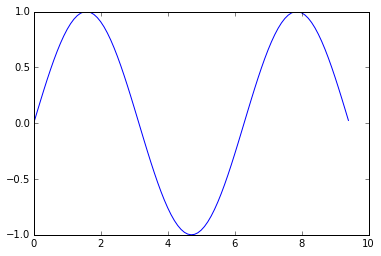
plt.plot(x, y)
plt.show()  # You must call plt.show() to make graphics appear.

Запуск этого кода приводит к следующему графику:

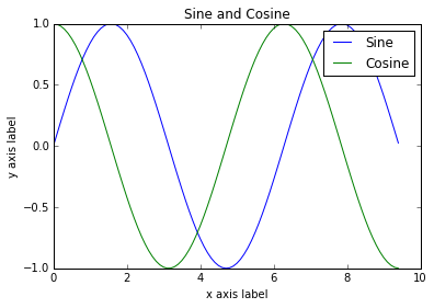
Приложив немного дополнительной работы, мы можем легко нарисовать несколько линий одновременно и добавить заголовок, легенду и метки оси:

import numpy as np
import matplotlib.pyplot as plt

# Compute the x and y coordinates for points on sine and cosine curves
x = np.arange(0, 3 * np.pi, 0.1)
y_sin = np.sin(x)
y_cos = np.cos(x)

# Plot the points using matplotlib
plt.plot(x, y_sin)
plt.plot(x, y_cos)
plt.xlabel('x axis label')
plt.ylabel('y axis label')
plt.title('Sine and Cosine')
plt.legend(['Sine', 'Cosine'])
plt.show()

Вы можете прочитать намного больше о plotфункции в документации .

Андрос и Норрис

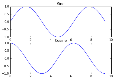
Вы можете нарисовать разные вещи на одной фигуре, используя subplotфункцию. Вот пример:

import numpy as np
import matplotlib.pyplot as plt

# Compute the x and y coordinates for points on sine and cosine curves
x = np.arange(0, 3 * np.pi, 0.1)
y_sin = np.sin(x)
y_cos = np.cos(x)

# Set up a subplot grid that has height 2 and width 1,
# and set the first such subplot as active.
plt.subplot(2, 1, 1)

# Make the first plot
plt.plot(x, y_sin)
plt.title('Sine')

# Set the second subplot as active, and make the second plot.
plt.subplot(2, 1, 2)
plt.plot(x, y_cos)
plt.title('Cosine')

# Show the figure.
plt.show()

Вы можете прочитать намного больше о subplotфункции в документации .

Картинки

Вы можете использовать imshowфункцию для показа изображений. Вот пример:

import numpy as np
from scipy.misc import imread, imresize
import matplotlib.pyplot as plt

img = imread('assets/cat.jpg')
img_tinted = img * [1, 0.95, 0.9]

# Show the original image
plt.subplot(1, 2, 1)
plt.imshow(img)

# Show the tinted image
plt.subplot(1, 2, 2)

# A slight gotcha with imshow is that it might give strange results
# if presented with data that is not uint8. To work around this, we
# explicitly cast the image to uint8 before displaying it.
plt.imshow(np.uint8(img_tinted))
plt.show()